This blog post will give you a gentle introduction to the use of the elytica Interpreter. The benefits of using it to solve real-world practical optimization problems will become clear as we work through the various tutorials.
Logging in and starting your project
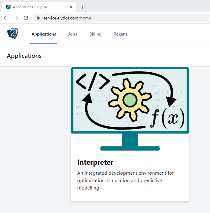
To sign up for a free trial account (which never expires by the way!!), register at https://service.elytica.com. The following screen will appear with a first time successful login:

By clicking on the Interpreter application icon, you will be redirected to compute.elytica.com, the home of the elytica Interpreter.
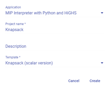
This means that the next time you want to make use of the Interpreter, you can simply point your browser to compute.elytica.com and log in. For the first time log in, you will be welcomed by the following form which will allow you to create your first optimization model (we took the liberty of pre-populating it for you).

For your first project we have selected “MIP Interpreter with Python and HiGHS” as the “Application”. This will allow you to solve Mixed Integer linear Programming (MIP) problems with the open-source solver HiGHS, and you will be able to make use of Python for general data manipulation tasks. Depending on your subscription type, other scripting language and solver combinations may be available, e.g.
- MIP Interpreter with Lua and Cbc
- MIP Interpreter with Python and Gurobi
- MIP Interpreter with Lua and CPLEX
- MIP Interpreter with Python and Cbc, etc.
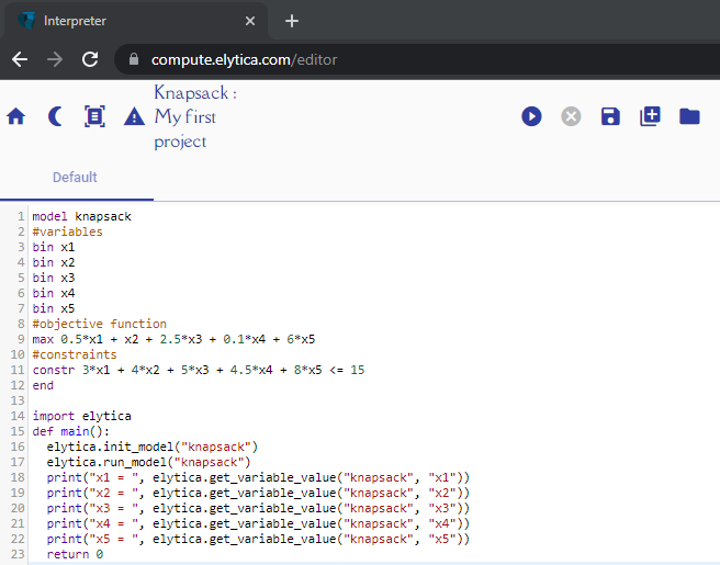
When you click on “Create” you will be transferred to the following editor screen

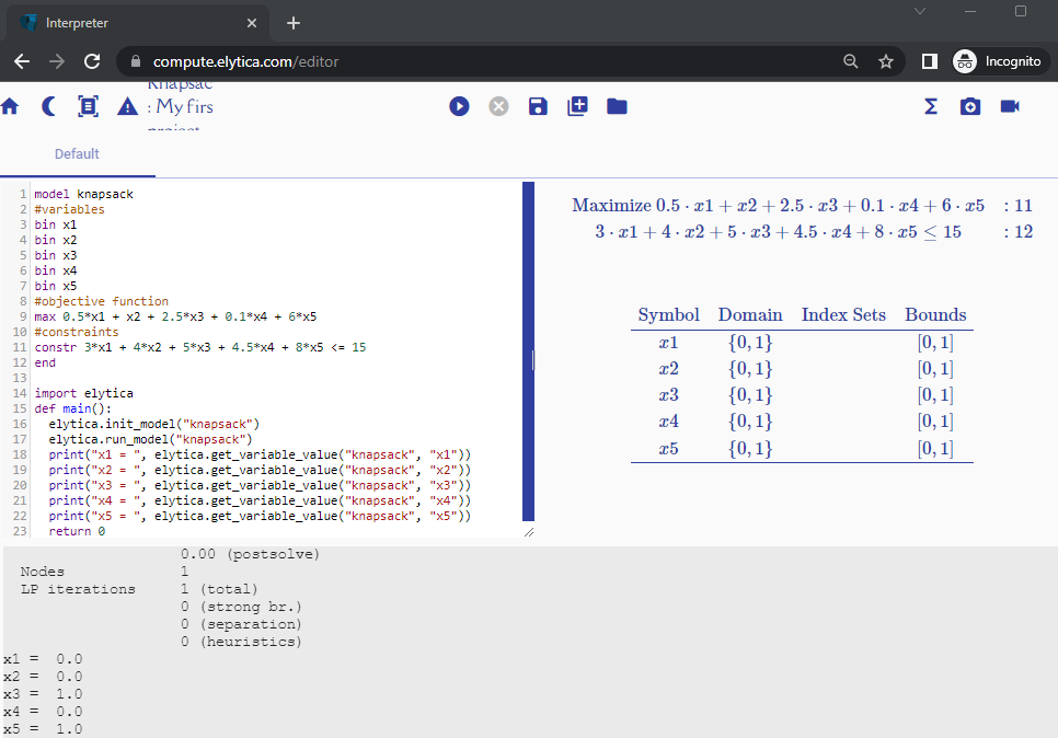
By pressing the run button ![]() output appear on the right-hand side of the screen (rendering of the mathematical model), as well as the bottom of the screen (output produced by solving the optimization problem):
output appear on the right-hand side of the screen (rendering of the mathematical model), as well as the bottom of the screen (output produced by solving the optimization problem):

Syntax used for capturing mathematical formulations
Before we start interacting with the elytica Interpreter, let us review the formulation of the standard knapsack problem. The input is a list of items and associated with each item is a value and a weight.
| Item | Value ($) | Weight (kg) |
|---|---|---|
| 1 | 0.5 | 3 |
| 2 | 1 | 4 |
| 3 | 2.5 | 5 |
| 4 | 0.1 | 4.5 |
| 5 | 6 | 8 |
Let’s assume we have a knapsack (container) which has a capacity of 15kg. Then, the objective of solving the knapsack problem is to identify which items to pack into the knapsack that would provide you with the best dollar value in total, keeping in mind that the knapsack has a finite capacity.
To capture this logic mathematically, let us introduce binary decision variables x_1, x_2, \dots, x_5. An item will be packed into the knapsack if its corresponding decision variable takes on a value of 1 as part of the solution, and 0 otherwise. Mathematically we can formulate the problem as
\text{maximize} \ 0.5x_1+x_2+2.5x_3+0.1x_4+6x_5
\\\text{subject to} \ 3x_1+4x_2+5x_3+4.5x_4+8x_5 \le 15
Optimization problems are captured on the elytica platform in terms of variables, an objective function and constraints, in the space between the key words model [model_name] and end. Statements followed by a # are treated as comments by the Interpreter.
model knapsack

# variables, objective function, and constraints defined here

end
First, binary decision variables are declared by using the binary keyword.
binary x1
binary x2
binary x3
binary x4
binary x5
It is, of course, also possible to declare variables of other types, depending on the type of problem you are trying to formulate. Below are examples of other variable type declarations with different bound conditions.
var 0 <= y1 <= 100 #continuous variable between 0 and 100
int 0 <= y2        #integer variable greater or equal than 0
var y3             #unrestricted continuous variable
The objective function is defined by the maximize or minimize keywords. The abbreviations max or min will also be acceptable to the interpretation engine.
max 0.5*x1 + x2 + 2.5*x3 + 0.1*x4 + 6*x5Note that, although it is mathematically acceptable to write down the product of, for example 0.5 and the variable x_1 as 0.5x_1, we need to make it clear to the Interpretation engine that we are multiplying a constant with a variable by using the multiplication operator , for example 0.5*x1.
The knapsack capacity constraint is added to the model formulation by using the constraint (or the abbreviation constr) keyword:
constr 3*x1 + 4*x2 + 5*x3 + 4.5*x4 + 8*x5 <= 15You are now ready to solve your first optimization model on the elytica platform!! If you have followed all the steps above, your model code should look like this:
model knapsack
bin x1
bin x2
bin x3
bin x4
bin x5
max 0.5*x1 + x2 + 2.5*x3 + 0.1*x4 + 6*x5
constr 3*x1 + 4*x2 + 5*x3 + 4.5*x4 + 8*x5 <= 15
end
But before you hit the run button, there are still some additional configurations required that will allow the model to be solved and the solution to be printed to the screen. And this is where it gets even more interesting! Recall that you created your project based on the application selection ” MIP Interpreter with Python and HiGHS”. Yes, you guessed it – these extra configuration settings will be done in Python:
import elytica
def main():
  elytica.init_model("knapsack")
  elytica.run_model("knapsack")
  print("x1 = ", elytica.get_variable_value("knapsack", "x1"))
  print("x2 = ", elytica.get_variable_value("knapsack", "x2"))
  print("x3 = ", elytica.get_variable_value("knapsack", "x3"))
  print("x4 = ", elytica.get_variable_value("knapsack", "x4"))
  print("x5 = ", elytica.get_variable_value("knapsack", "x5"))
  return 0
First, the elytica Python package needed to solve the knapsack model is imported. In the main function, the knapsack model is initialized and solved, by explicitly referencing the name of the model. To print the solution values for the binary decision variables x_1, x_2, \dots, x_5, the elytica function get_variable_value() is used.
